AI in Rust: 01 Use Jupyter to Learn Rust
Intro
Everybody, Ok, most people, says that Rust is difficult, I don’t think so. Although Rust may be a little harder than Python, we can learn Rust in the same way as Python – by using Jupyter.
In this article I will show you how to write Rust code in interactive mode, especially in the data science scenarios.
Installation
First, you need to install `Jupyter`, the interactive notebook, developed by Python. You can do it by (I assume that you have installed Python before):
pip install jupyterlab
Remember to check whether the installation is successful, please run this command:
jupyter lab
You would see a Web UI, close it right now.
After that, we need to install `Evcxr Jupyter Kernel`, which is the Rust kernel extension of Jupyter. Do it by (I assume that you have installed Rust on your machine before):
cargo install --locked evcxr_jupyter
evcxr_jupyter --install
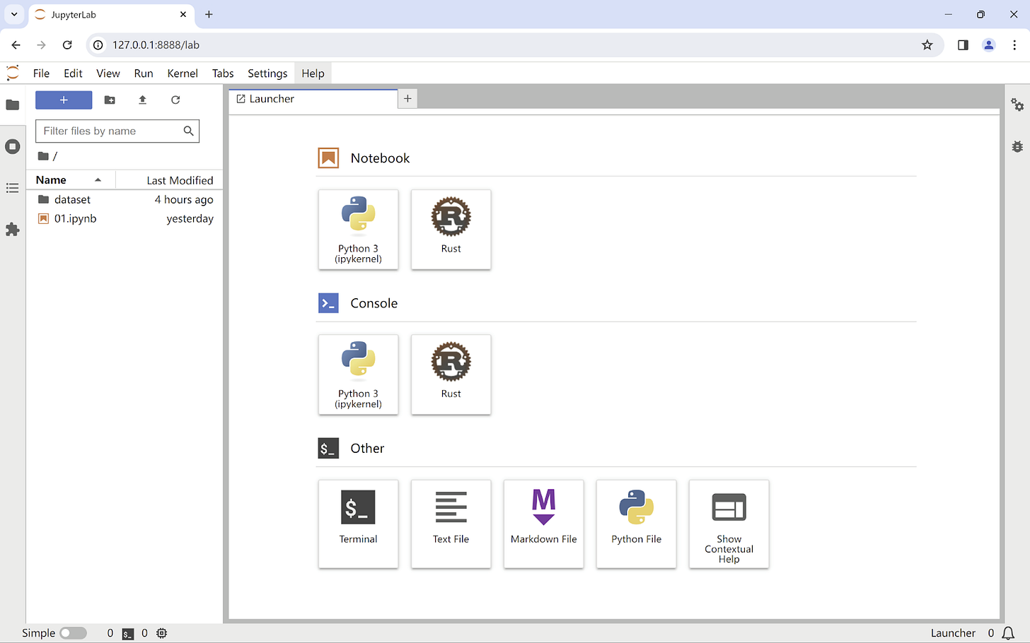
After everything is done, start the jupyter UI once again, you will look at something like:
Congrats, we have the Rust logo on the launcher panel.
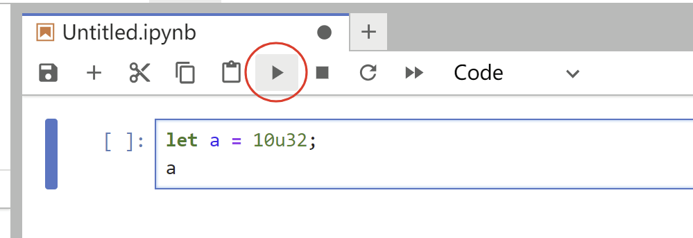
Just click the Rust square under the Notebook section, we get:
Everything ready, let’s go.
Basic Operations
To practice this tutorial, I suggest that you have the basic background of Rust language.
Let’s start by testing basic variable binding,
Output as:
The output is printed at the next line below the Rust code, yes, interactively.
Let’s continue.
It seems everything is going well. We can now proceed to more complex tasks.
We will utilize the set of three tools for data science: polars, ndarray and plotters to learn how to use Rust to work with data analysis.
Use Polars to Analyze Dataset
In this tutorial, I’m going to choose the Titanic dataset for example to illustrate how convenient Rust is.
According to New Bing: “The Titanic dataset is a popular dataset used in data science and machine learning. It contains information about the passengers on the Titanic, including details like age, sex, class, fare, and whether or not they survived the disaster. This dataset is often used for predictive modeling exercises, such as predicting whether a passenger would have survived based on their characteristics. It’s a classic dataset for beginners in data analysis and machine learning, and is widely used in Kaggle competitions.”
We can download the Titanic dataset from here, and move it to `dataset/` subdirectory.
Add dependencies:
:dep ndarray = {version = "0.15.6"}
:dep polars = {version = "0.35.4", features = ["describe", "lazy", "ndarray"]}
:dep plotters = { version = "0.3.5", default_features = false, features = ["evcxr", "all_series", "all_elements"] }
Show dependencies:
:show_deps
Output:
ndarray = {version = "0.15.6"}
plotters = { version = "0.3.5", default_features = false, features = ["evcxr", "all_series", "all_elements"] }
polars = {version = "0.35.4", features = ["describe", "lazy", "ndarray"]}
Read the dataset into polars memory:
use polars::prelude::*;
use polars::frame::DataFrame;
use std::path::Path;

fn read_data_frame_from_csv(
 csv_file_path: &Path,
) -> DataFrame {
 CsvReader::from_path(csv_file_path)
    .expect("Cannot open file.")
    .has_header(true)
    .finish()
    .unwrap()
}

let titanic_file_path: &Path = Path::new("dataset/titanic.csv");
let titanic_df: DataFrame = read_data_frame_from_csv(titanic_file_path);
Inspect the shape of this data:
titanic_df.shape()
Output:
(891, 12)
DataFrame is the basic structure in polars, it’s the same as it in Python Pandas, you can look at it as a 2-dimensions datasheet table with a named header for each column.
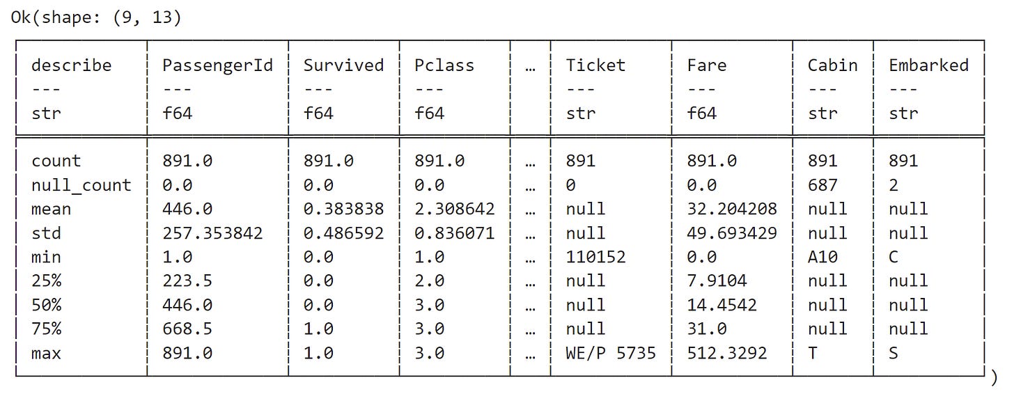
Overview the basic statistic information of this dataset:
titanic_df.describe(None)
Output:
We can see that there are some null cells in this dataset.
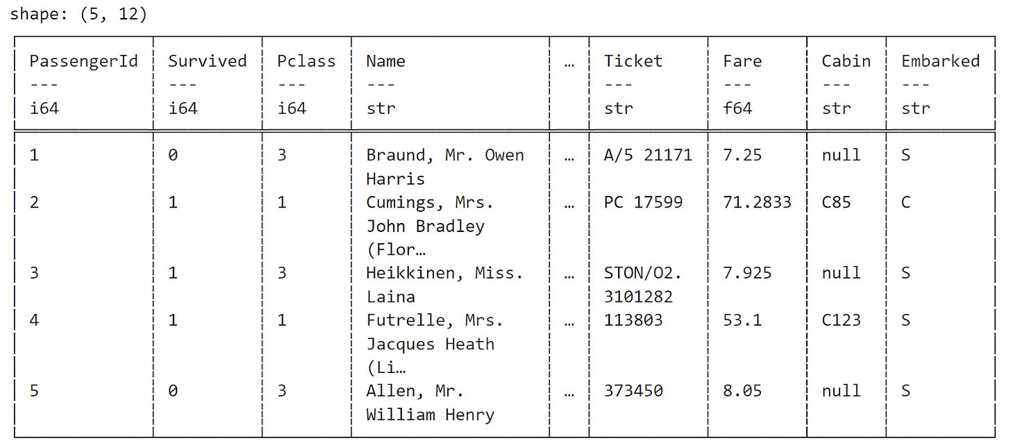
Inspect the head 5 lines:
titanic_df.head(Some(5))
Output:
Some columns collapsed, let’s inspect how many columns actually, use `.schema()` to get column names.
titanic_df.schema()
Output:
Schema:name: PassengerId, data type: Int64
name: Survived, data type: Int64
name: Pclass, data type: Int64
name: Name, data type: String
name: Sex, data type: String
name: Age, data type: Float64
name: SibSp, data type: Int64
name: Parch, data type: Int64
name: Ticket, data type: String
name: Fare, data type: Float64
name: Cabin, data type: String
name: Embarked, data type: String
Check how many people survived:
titanic_df["Survived"].value_counts(true, true)
Output:
Ok(shape: (2, 2)
┌──────────┬───────┐
│ Survived ┆ count │
│ ---      ┆ ---   │
│ i64      ┆ u32   │
╞══════════╪═══════╡
│ 0        ┆ 549   │
│ 1        ┆ 342   │
└──────────┴───────┘)
To check the gender distribution:
titanic_df["Sex"].value_counts(true, true)
Output:
Ok(shape: (2, 2)
┌────────┬────────┐
│ Sex    ┆ counts │
│ ---    ┆ ---    │
│ str    ┆ u32    │
╞════════╪════════╡
│ male   ┆ 577    │
│ female ┆ 314    │
└────────┴────────┘)
You can continue to do more complex EDA (Exploratory Data Analysis) on `titanic_df` DataFrame.
Use Plotters to Visualize Your Data
Next we can use the `plotters` crate to visualize our output data.
Import symbols:
use plotters::prelude::*;
Draw bar diagram:
evcxr_figure((640, 480), |root| {
 let drawing_area = root;
 drawing_area.fill(&WHITE).unwrap();

 let mut chart_context = ChartBuilder::on(&drawing_area)
    .caption("Titanic Dataset", ("Arial", 30).into_font())
    .x_label_area_size(40)
    .y_label_area_size(40)
    .build_cartesian_2d((0..1).into_segmented(), 0..800)?;

 chart_context.configure_mesh()
    .x_desc("Survived?")
    .y_desc("Number").draw()?;

 let data_s: DataFrame = titanic_df["Survived"].value_counts(true, true).unwrap().select(vec!["counts"]).unwrap();
 let mut data_source = data_s.to_ndarray::<Int32Type>(IndexOrder::Fortran).unwrap().into_raw_vec().into_iter();

 chart_context.draw_series((0..).zip(data_source).map(|(x, y)| {
    let x0 = SegmentValue::Exact(x);
    let x1 = SegmentValue::Exact(x + 1);
    let mut bar = Rectangle::new([(x0, 0), (x1, y)], BLUE.filled());
    bar.set_margin(0, 0, 30, 30);
    bar
 }))
 .unwrap();

 Ok(())
}).style("width:60%")
Display:
The code seems lengthy and tedious, it’s better to encapsulate a simple API to do it in plotters. Core problems are that 1. too many configuration items, 2. and complex type conversions.
Plotters support various figures, plots, and charts, you can think of plotters as the counterpart of Python matplotlib in the Rust ecosystem, but it still has some ways to go to match the ease of usage of matplotlib.
For more information about plotters, please visit: https://docs.rs/plotters/latest/plotters/
Next we will introduce the matrix manipulation library `ndarray`.
Use Ndarray to Manipulate Matrix
DataFrame has a method to convert itself to Ndarray’s multiple dimension matrix. For example:
let a = UInt32Chunked::new("a", &[1, 2, 3]).into_series();
let b = Float64Chunked::new("b", &[10., 8., 6.]).into_series();

let df = DataFrame::new(vec![a, b]).unwrap();
let ndarray = df.to_ndarray::<Float64Type>(IndexOrder::Fortran).unwrap();
println!("{:?}", ndarray);
Will output:
[[1.0, 10.0],
 [2.0, 8.0],
 [3.0, 6.0]], shape=[3, 2], strides=[1, 3], layout=Ff (0xa), const ndim=2
We can use this matrix type to do complex matrix operations by `ndarray` crate.
Import symbols:
use ndarray::*;
Create a 2x3 matrix:
array![[1.,2.,3.], [4.,5.,6.]]
Output:
[[1.0, 2.0, 3.0],
 [4.0, 5.0, 6.0]], shape=[2, 3], strides=[3, 1], layout=Cc (0x5), const ndim=2
Create a range:
Array::range(0., 10., 0.5)
Output:
[0.0, 0.5, 1.0, 1.5, 2.0, 2.5, 3.0, 3.5, 4.0, 4.5, 5.0, 5.5, 6.0, 6.5, 7.0, 7.5, 8.0, 8.5, 9.0, 9.5], shape=[20], strides=[1], layout=CFcf (0xf), const ndim=1
Create a range with equal inner space:
Array::linspace(0., 10., 18)
Output:
[0.0, 0.5882352941176471, 1.1764705882352942, 1.7647058823529411, 2.3529411764705883, 2.9411764705882355, 3.5294117647058822, 4.11764705882353, 4.705882352941177, 5.294117647058823, 5.882352941176471, 6.470588235294118, 7.0588235294117645, 7.647058823529412, 8.23529411764706, 8.823529411764707, 9.411764705882353, 10.0], shape=[18], strides=[1], layout=CFcf (0xf), const ndim=1
Create a 3x4x5 matrix (also called ‘tensor’ in machine learning):
Array::<f64, _>::ones((3, 4, 5))
Output:
[[[1.0, 1.0, 1.0, 1.0, 1.0],
  [1.0, 1.0, 1.0, 1.0, 1.0],
  [1.0, 1.0, 1.0, 1.0, 1.0],
  [1.0, 1.0, 1.0, 1.0, 1.0]],

 [[1.0, 1.0, 1.0, 1.0, 1.0],
  [1.0, 1.0, 1.0, 1.0, 1.0],
  [1.0, 1.0, 1.0, 1.0, 1.0],
  [1.0, 1.0, 1.0, 1.0, 1.0]],

 [[1.0, 1.0, 1.0, 1.0, 1.0],
  [1.0, 1.0, 1.0, 1.0, 1.0],
  [1.0, 1.0, 1.0, 1.0, 1.0],
  [1.0, 1.0, 1.0, 1.0, 1.0]]], shape=[3, 4, 5], strides=[20, 5, 1], layout=Cc (0x5), const ndim=3
Create a zero initial matrix:
Array::<f64, _>::zeros((3, 4, 5))
Output:
[[[0.0, 0.0, 0.0, 0.0, 0.0],
  [0.0, 0.0, 0.0, 0.0, 0.0],
  [0.0, 0.0, 0.0, 0.0, 0.0],
  [0.0, 0.0, 0.0, 0.0, 0.0]],

 [[0.0, 0.0, 0.0, 0.0, 0.0],
  [0.0, 0.0, 0.0, 0.0, 0.0],
  [0.0, 0.0, 0.0, 0.0, 0.0],
  [0.0, 0.0, 0.0, 0.0, 0.0]],

 [[0.0, 0.0, 0.0, 0.0, 0.0],
  [0.0, 0.0, 0.0, 0.0, 0.0],
  [0.0, 0.0, 0.0, 0.0, 0.0],
  [0.0, 0.0, 0.0, 0.0, 0.0]]], shape=[3, 4, 5], strides=[20, 5, 1], layout=Cc (0x5), const ndim=3
Sum rows and columns:
let arr = array![[1.,2.,3.], [4.,5.,6.]];
Sum by row:
arr.sum_axis(Axis(0))
Output:
[5.0, 7.0, 9.0], shape=[3], strides=[1], layout=CFcf (0xf), const ndim=1
Sum by column:
arr.sum_axis(Axis(1))
Output:
[6.0, 15.0], shape=[2], strides=[1], layout=CFcf (0xf), const ndim=1
Sum all elements:
arr.sum()
Output:
21.0
Transpose:
arr.t()
Output:
[[1.0, 4.0],
 [2.0, 5.0],
 [3.0, 6.0]], shape=[3, 2], strides=[1, 3], layout=Ff (0xa), const ndim=2
Dot multiplication:
arr.dot(&arr.t())
Output:
[[14.0, 32.0],
 [32.0, 77.0]], shape=[2, 2], strides=[2, 1], layout=Cc (0x5), const ndim=2
Square root:
arr.mapv(f64::sqrt)
Output:
[[1.0, 1.4142135623730951, 1.7320508075688772],
 [2.0, 2.23606797749979, 2.449489742783178]], shape=[2, 3], strides=[3, 1], layout=Cc (0x5), const ndim=2
We will end here, ndarray is a super-powerful tool, you can use it to perform any tasks about matrices and linear algebra.
Recap
In this article, I illustrate how to use Jupyter to learn Rust interactively. Jupyter is a super tool for data scientists (or students), we can finish exploratory data analysis tasks in Jupyter using Rust now. Polars, plotters and ndarray are powerful toolsets to help us deal with the data analysis and data preprocessing work, which is a prerequisite for the following machine learning task.


It's late Feb 2025.
Everything still working well
Great guide
Thanks for sharing this. It was very simple and beginner friendly. I hope you upload some major project tutorial in rust jupyter in the near future.